How to Use COUNTIF in Google Sheets

Functions and formulas help us perform all sorts of tasks, actions, and calculations in spreadsheets. If you have a Google Sheet where you want to count a number of items that meet a specific condition, you need the COUNTIF function.

Using COUNTIF in Google Sheets, you can save time and manual work from counting the items “by hand.” Simply enter the data range and criterion in the formula to get your result in seconds.

About the Google Sheets COUNTIF Function

COUNTIF is a variation of the COUNT function that lets you count cells in a dataset that meet a particular condition. As examples, you may want to count the number of students with a certain GPA, employees who’ve worked a specific number of years with your company, or even car models that begin with a particular letter. With COUNTIF, you have many possibilities to count the data you need quickly.

The syntax for the function’s formula is COUNTIF(range, condition) with these options for the condition argument:

• Use a question mark (?) as a wildcard to match a single character.
• Use an asterisk (*) to match zero or more adjacent characters.
• To match a question mark or asterisk, place a tilde (~) before it, for example, ~? or ~*.
• Use the equal sign (=), greater than (>), and less than (<) symbols to compare number equality.
• Enclose a character string in quotation marks.

How to Use COUNTIF in Google Sheets

The best way to explain how to use a function and its formula is to see them in action. Let’s look at a handful of formula examples for COUNTIF in Google Sheets.

Count Items Greater Than or Equal to a Value

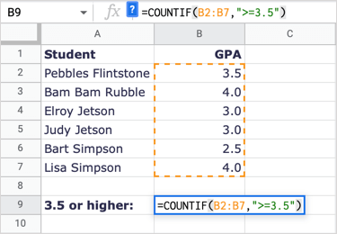
Using a student grade example, we’ll count the number of students who have a GPA greater than or equal to 3.5.

Select the cell where you want the result, this is where you’ll type the formula. Enter the following formula making sure to begin with the equal sign and include a comma between the arguments:

=COUNTIF(B2:B7,”>=3.5”)

To break down the formula, B2:B7 is the range of cells and “>=3.5” is the condition for greater than or equal to 3.5.

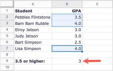
As you can see, we receive a result of 3 which is correct. There are three students that have a GPA of 3.5 or higher.

Related: Having trouble with formulas? Check out our guide to troubleshooting Google Sheets formula parse errors.

Count Items Less Than a Value

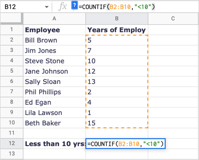
In this next example, let’s count the number of employees who have worked for us less than 10 years.

Select the cell where you want the results and enter the following formula:

=COUNTIF(B2:B10,”<10″)

To break down the formula, B2:B10 is the data range and “<10” is the condition for less than 10.

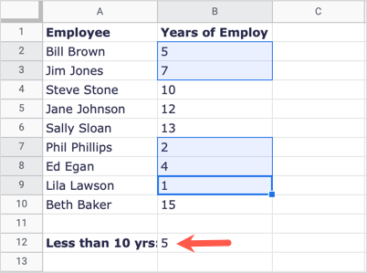
We receive 5 as our result which is correct. Notice that Steve Stone has worked for us for 10 years, but he is not part of the result because 10 is not less than 10.

Count Items That Start With a Letter

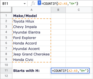
For another example, let’s count the number of makes of cars, not models, that start with the letter H.

Select the cell where you want the formula result and type the following:

=COUNTIF(A2:A9,”H*”)

To break down this formula, A2:A9 is our range and “H*” is the condition for the first letter H and the asterisk wildcard for any following letters.

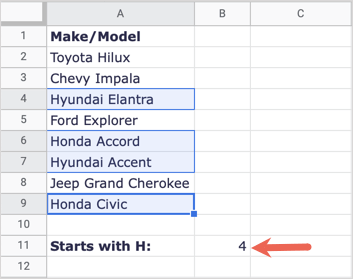
Here, we receive a result of 4 which is correct; we have four car makes that start with the letter H.

Count Items Matching Cell Values

Maybe the condition you want to match already exists in another cell. You can use this by placing the string in quotation marks, adding an ampersand (&), and entering the cell reference.

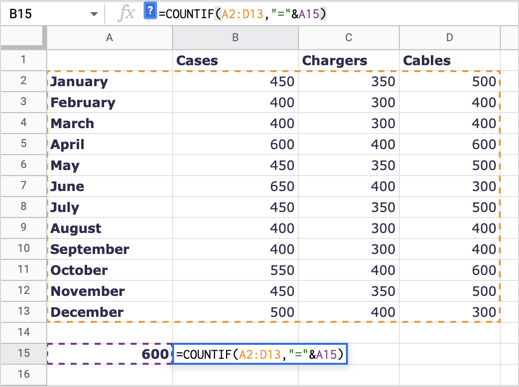
Here, we’ll count the number of times that the value in cell A15 (600) appears in our dataset.

Select the cell where you want the result and enter this formula:

=COUNTIF(A2:D13,”=”&A15)

Breaking down the formula, A2:D13 is the data range, “=” is the operator (string) in quotes, and &A15 is the value we want to match in cell A15.

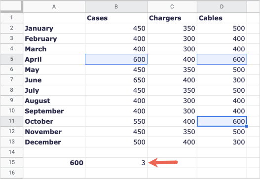
We receive 3 as our result which is correct, we have three items matching 600.

Count Items Matching Text Values

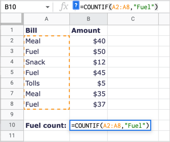
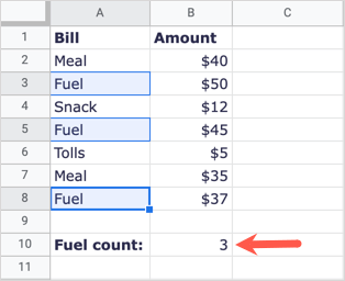
For one final example, you might want to count the number of cells with specific text. Let’s count the total number of expenses for Fuel.

Select the cell where you want the result and enter this formula:

=COUNTIF(A2:A8,”Fuel”)

To break down this formula, A2:A8 is the data range and “Fuel” is the condition to match.

We receive our result of 3 which is correct. Note: COUNTIF is not case sensitive, so you could enter “FUEL” or “fuel” for the text string and receive the same result.

When you need to count a number of items but only those that meet your criterion, the COUNTIF function in Google Sheets works like a dream.

If you want to count items that match multiple criteria, you can use the COUNTIFS function. Check out our tutorial for using COUNTIFS along with similar functions in Microsoft Excel and apply the same formula structure in Google Sheets.