How to Add or Remove Hyperlinks in Google Sheets

Adding a hyperlink is one of the best ways to access something in your spreadsheet quickly. You can link to a cell, cell range, other sheet, and even a web page in Google Sheets.

We will show you how to add hyperlinks to your worksheet and remove links in Google Sheets that you no longer want.

Link to a Cell or Cell Range

If you have a large Google spreadsheet full of data and want to visit a single cell or cell range frequently, you can easily create a link to it.

1. Select the cell where you want to place the hyperlink. If the cell contains text, that text will be linked. You can also add the text you want when you create the link.
2. Do one of the following to insert the link:
3. Right-click and pick Insert Link.
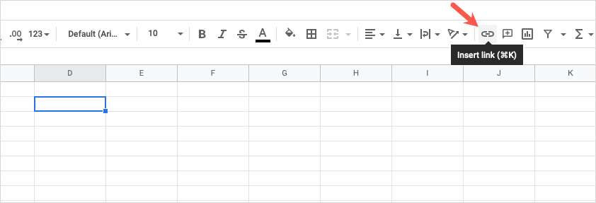
4. Select the Insert Link button in the toolbar.
5. Choose Insert > Link from the menu.

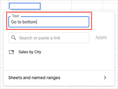
6. When the Insert Link box appears, you’ll see the cell contents to be linked in the Text box at the top. If the cell is blank, you can enter text in that box to connect to the link.

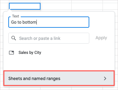
7. Navigate to the bottom of the pop-up box and pick Sheets and named ranges.

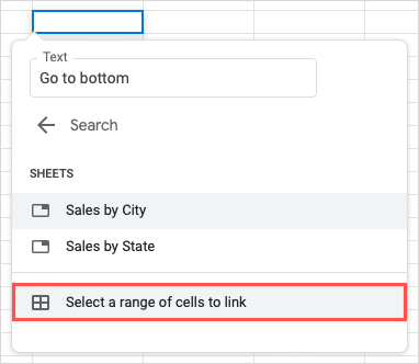
8. Go to the bottom of the subsequent screen and pick Select a range of cells to link.

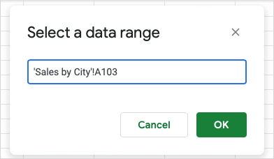
9. Either enter the cell reference or cell range starting with the sheet name in the following dialog box or use your cursor to select the cell or range to automatically populate the box.
10. Confirm the cell or range and select OK.

You’ll then see the linked text within the cell. Select the cell and use the link in the preview to head to the cell or cell range.

Link to a Named Cell Range

If you use named ranges in your sheet, this gives you another linking option.

1. Follow Steps 1 through 3 above to select the cell, open the Insert Link box, and optionally adjust or add the link text.
2. Go to the bottom of the pop-up box and pick Sheets and named ranges.
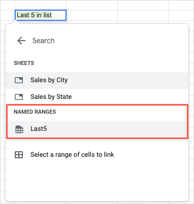
3. If necessary, scroll down the next screen in the box to the Named Ranges section and pick the range.

4. When the link to the named range appears in the cell, use Enter or Return to save it.

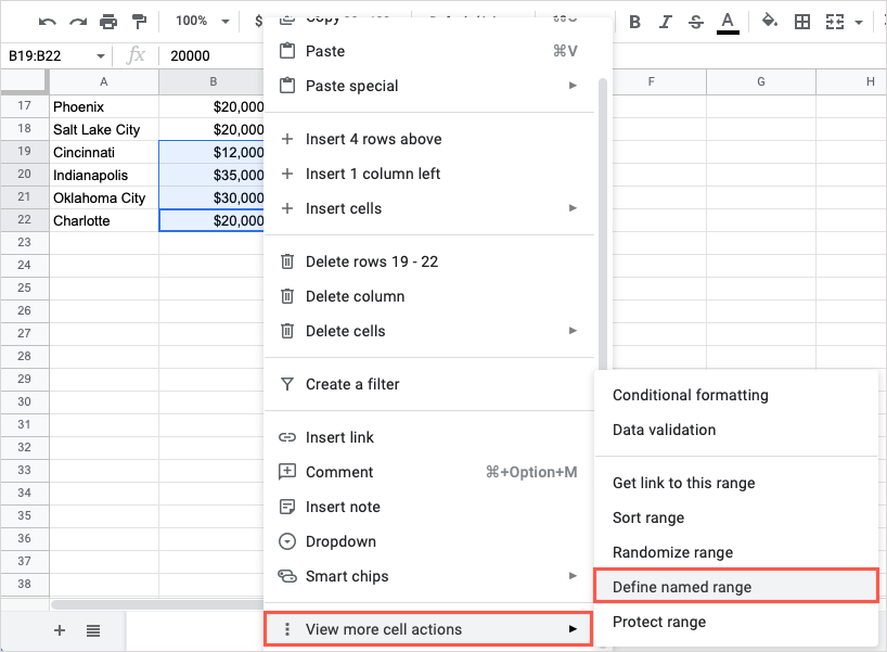
If you don’t see the named range in the list, it’s likely that it wasn’t named already. To do so, select the range of cells, right-click, and pick View more cell actions > Define named range.

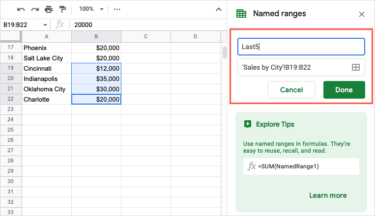
When the Named Ranges sidebar appears on the right, enter a name for the range and select Done.

You can then follow the previous steps to link to that named range.

Link to Another Sheet

If you want to link to another spreadsheet in your Google Sheets workbook, this is a handy way to jump right to it when needed.

1. Follow Steps 1 through 3 from earlier.
2. Go to the bottom of the pop-up box and pick Sheets and named ranges.
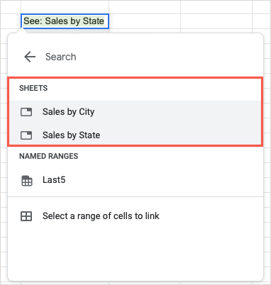
3. Head to the Sheets section and pick the sheet name.

4. When the link to the sheet appears in the cell, use Enter or Return to save it.

Link to a Web Page

When you want to link to a website or a particular web page, you have few different ways to do so in Google Sheets.

Use the Paste Action

Probably the simplest way to insert a web link in your sheet is by copying and pasting the URL.

1. Go to the address bar in your web browser and copy the link. You can do this by selecting the URL, right-clicking, and picking Copy.

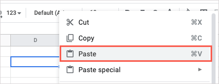
2. Return to Google Sheets and select the cell where you want the link, right-click, and pick Paste.

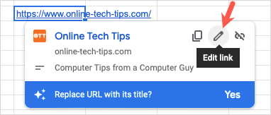
3. You’ll then see the hyperlink in the cell. If you want to edit the name rather than display the URL, select the cell to display the link preview and pick the Edit link button (pencil icon).

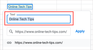
4. Enter the name in the Text box and select Apply.

Use the Insert Link Feature

Another way to link to a site or page is using the Insert Link feature described earlier.

1. Select the cell where you want the link and do one of the following:
2. Right-click and pick Insert Link.
3. Select the Insert Link button in the toolbar.
4. Choose Insert > Link from the menu.
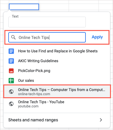
5. Search for, type, or paste the link into the Search or paste a link box.
6. Optionally add or edit the name in the Text box and select Apply.

Use the HYPERLINK Function

If you like using functions and formulas in Google Sheets, you can also use the HYPERLINK function to insert your link.

The syntax for the formula is “HYPERLINK(url, label)”, where only the URL is required. You can use the label argument for the text to link to the URL. Be sure to include both arguments within quotation marks.

To insert a link to Online Tech Tips, you would use this formula:

=HYPERLINK(“https://www.online-tech-tips.com”)

To insert a link to Online Tech Tips that has the label OTT, you’d use this formula instead:

=HYPERLINK(“https://www.online-tech-tips.com”,”OTT”)

Remove Hyperlinks in Google Sheets

If you decide later to remove hyperlinks you’ve added or import data or a sheet from elsewhere and don’t want the included links, you can remove them.

Remove a Single Link in a Sheet

Maybe you have a particular hyperlink you want to remove. You can do this in a snap. Do one of the following to remove an individual link:

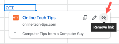
Select the cell containing the link and pick the Remove link button (broken link icon) in the preview.

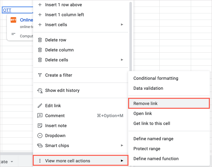
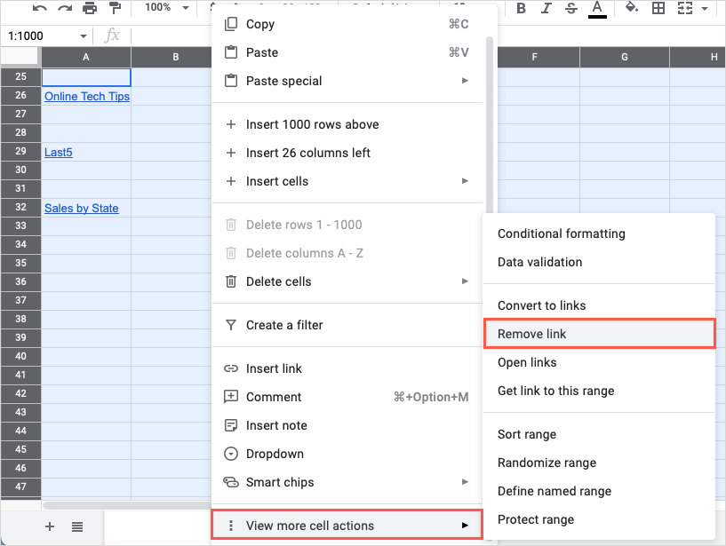
Right-click the cell with the link and move to View more cell actions > Remove link.

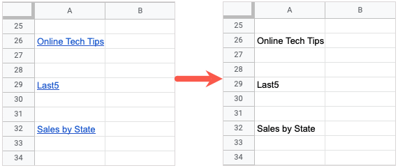
The hyperlink is removed, but the text for the link remains in the cell.

Remove All Links in a Sheet

Perhaps you have many links in your sheet. Rather than remove them one at a time, you can take care of them all in one fell swoop.

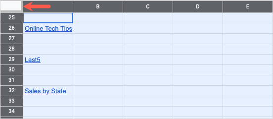
1. Select the entire sheet using the Select All button (square in the top-left corner). You can also use the keyboard shortcut Ctrl + A on Windows or Command + A on Mac.

2. Right-click anywhere in the sheet, move to View more cell actions, and pick Remove link.

3. You should then see all hyperlinks in your sheet vanish, but any text you used for the links remain.

When you want a fast way to jump to another cell, sheet, or web page, you can add hyperlinks in Google Sheets in various ways.

For other helpful productivity tips, look at how to use find and replace in Google Sheets.