Have there been times you set up your spreadsheet and then realized that a different layout would work better? You can easily convert rows to columns or vice versa in Google Sheets to display your data as you please.
With two ways to switch your rows and columns, you can use whichever is most comfortable for you. This includes the Paste Special feature and the TRANSPOSE function. If you’re ready to go, here’s how to use transpose in Google Sheets.

Convert Rows and Columns With Paste Special
A quick way to convert rows and columns is using the Paste Special feature in Google Sheets. With it, you simply copy the data and then paste it as transposed.
The nice thing about using this option is that if you have formatting like bold text or a fill color in your cells, that formatting applies to the pasted cells.
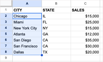
- Start by selecting the data you want to transpose. For example, we’ll convert our column of cities to a row.
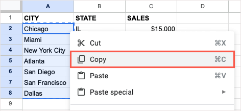
- Copy the data by doing one of the following:
- Select Edit > Copy from the menu.
- Right-click and choose Copy.
- Use the keyboard shortcut Ctrl + C on Windows or Command + C on Mac.
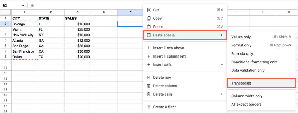
- Go to the cell where you want to paste the data, making sure you have enough space so that you don’t overwrite existing data.
- Either select Edit > Paste Special or right-click and move to Paste Special. Then, pick Transposed in the pop-out menu.
You should then see your selected cells pasted.
If you want to remove the original data after you paste it, you can delete it like any other data in your sheet.
Convert Rows and Columns With the TRANSPOSE Function
If you’re accustomed to using Google Sheets formulas, you can convert your rows or columns using the TRANSPOSE function and a simple formula.
Keep in mind that unlike the Paste Special feature above, existing text or cell formatting does not apply when you use the TRANSPOSE function.
The syntax for the formula is TRANSPOSE(range) with just one required argument for the range of cells you want to switch.
Go to the cell where you want the data transposed, making sure you have adequate space. Then, enter the following formula replacing the cell range with your own:
=TRANSPOSE(A2:G3)
Press Enter or Return and you should see your transposed data.
Again, you delete the original dataset after you use the TRANSPOSE formula to convert it if you like.
Convert Rows and Columns on Mobile
If you’re working with Google Sheets on your Android or iOS device, you can convert rows and columns there as well. While you can use the Paste Special feature or the TRANSPOSE function on Android, you can currently only use the function on iPhone.
Transpose on Android
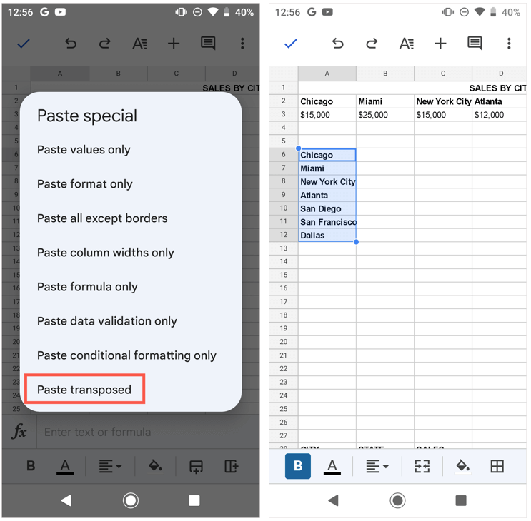
To switch rows or columns on Android, open your Google Sheet and follow these simple steps to use Paste Special.
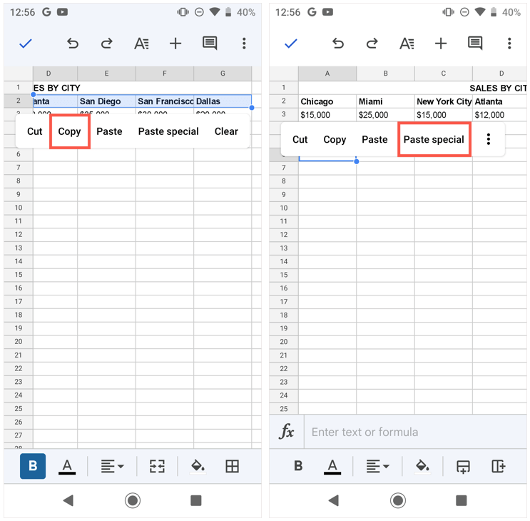
- Select the cells you want to transpose. You can drag through them using the blue dot on the bottom right corner. Then, tap to display the toolbar and choose Copy.
- Go to the cell where you want the converted rows or columns, tap, and select Paste special in the toolbar.
- When the Paste Special options appear, choose Paste transposed.
You’ll then see your converted rows or columns.
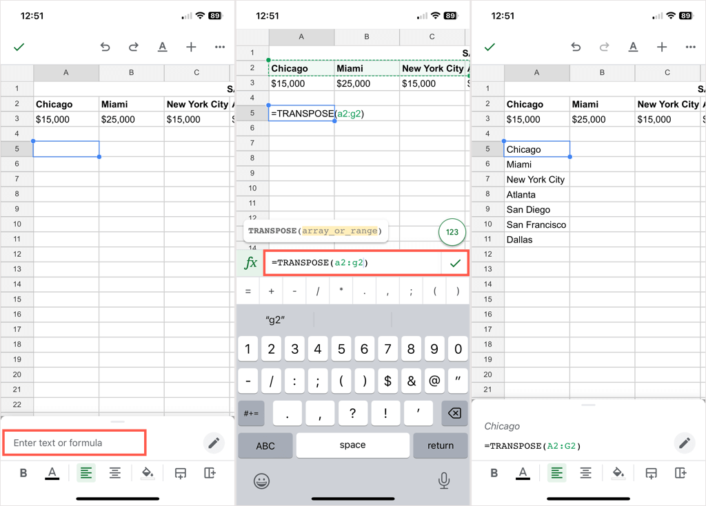
If you prefer to use the TRANSPOSE function on Android, follow the steps below as they are the same on iPhone.
Transpose on iPhone
As mentioned, you cannot use the Paste Special feature in Google Sheets on iPhone as of this writing. You can, however, use the TRANSPOSE function to switch your rows and columns.
- Go to the cell where you want the transposed cells.
- Type the formula into the text box at the bottom.
- Tap the green checkmark to apply the formula and you should see your converted rows or columns.
Converting rows to columns or the other way around is easy to do in Google Sheets. If you also use Microsoft Office, look at how to transpose data in Excel too!
